Confouning factors in event-related NIRS analysis
There has been growing interest in brain imaging applications of NIRS compared to functional magnetic resonance imaging (fMRI), mainly due to its higher temporal resolution, better cost-effectiveness and lower sensitivity to motion artifacts (Boas et al., 2004; Cui et al., 2011). FNIRS has been used to study cortical hemodynamics associated with transient neural activity triggered by external stimuli or endogenous neuronal transients such as interictal spikes (Plichta et al., 2007; Takeuchi et al., 2009; Osharina et al., 2010, 2016; Cui et al., 2011; Scarpa et al., 2013). Conventional averaging (CA) and the deconvolution method (DM) are two techniques commonly used to estimate the Hemodynamic Response Function (HRF) profile in event-related NIRS and fMRI studies (Hoshi and Tamura 1993; Kato et al. 1993; Villringer et al. 1993; Schroeter et al. 2004; Plichta et al. 2006; Koch et al., 2006). In this study, we investigated the performance and robustness of CA and DM for estimation of the HRF profile from simulated and experimental NIRS data and to explore the extent to which the estimated profile is biased by each of the aforementioned confounding factors in slow and rapid event-related designs. These simulations were designed by confounding NIRS signals by the inclusion of event sequences generated using stochastic or deterministic processes, corruption by physiological and instrumental noise under different SNR, corruption by noise phase-locked to event timing, the inclusion of temporal correlation in NIRS background activity, and the use of temporal filtering. The simulations were conducted with both synthesized and real resting-state NIRS data including physiological components, random noise, and experimental event sequences. We also investigated the nature of the experimental sequences of spikes recorded from a rat model of focal epilepsy and their effect on the performance and efficiency of these two techniques.
Our simulations consisted of forward modeling and HRF estimation procedures. For forward modeling, we used a linear model-based approach to simulate NIRS signals mimicking the temporal structure and complexities of real event-related NIRS data. In our basic forward model, any given event sequence S(t) was mapped to the NIRS signal Y(t) by using the following equation:
Y=α.(S*H)+N= α.Hs+N (1)
Where H is the hemodynamic response function, Hs is the simulated hemodynamic signal, and N is the additive components including physiological baseline fluctuations, nuisance, and other noises, α is the scaling factor, and ‘*’ is the linear convolution operator. The scaling factor was chosen to yield SNR values ranging from -20 dB to +20 dB in order to simulate the lowest and highest SNR levels in real NIRS data. Event sequences were simulated by stochastic or deterministic event generation processes. The timing of events was modeled as binary-valued sequences, where a value of 1 indicated the occurrence of an event, and a value of 0 indicated the absence of event (Bush and Cisler, 2013). We used the canonical hemodynamic response function as the actual response (H in Eq. (1)) of the hemodynamic system to event presentation. Additive components (N) were modeled as:
N= Xpc + Aε . f(ε) (2)
Where Xpc included baseline physiological fluctuations and nuisance parts, and ε was the uncorrelated (instrumental and measurement) noise term. In all simulations, Aε was the scaling factor for instrumental noise. f was the function defined on the basis of the requirements of each simulation. We included six frequency bands associated with particular biological mechanisms including spontaneous low-frequency oscillations, respiration, and cardiac pulsation (Majeed et al., 2009). We then modeled Xpc as:
Xpc = AULf . NULf+ AVLf . NVLf+ ALFlb . NLFlb+ ALFub . NLFub+ ARf . NRf +ACf . NCf (3)
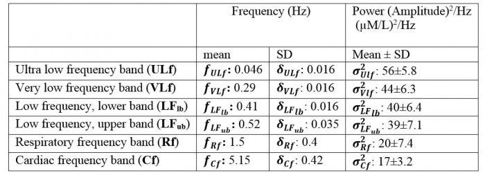
Where N and A refer to the physiological components and their amplitudes (see Table 1 for the definition and range of spectral power and frequency changes). We then synthesized the activation-free baseline physiological fluctuations and noise components of the NIRS signals using the parameters determined above. The spectral characteristics of the NIRS signals were therefore replicated by specifying a multimodal spectrum composed of the sum of six Gaussian functions (McSharry et al., 2003).
Table 1. Mean and standard deviation (SD) of the frequency and spectral power of the experimental physiological components
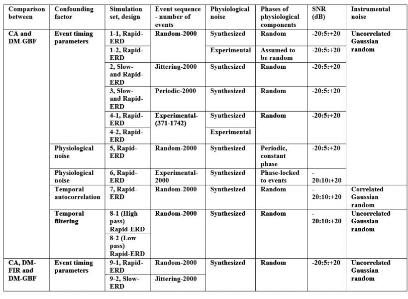
CA and DM were then used to estimate the time-course of the hemodynamic response for each synthesized NIRS data set. Table 2 summarizes the key features of the simulation sets generated in the study. A total of 3,570 simulations were performed for all nine simulation sets.
Table 2. Key features of the simulation sets. ERD: event-related design; CA: conventional averaging; DM-GBF: deconvolution model based on gamma basis functions; DM-FIR: deconvolution model based on FIR basis functions.
Our results demonstrated that DM was much less sensitive to confounding factors than CA. Event timing (Figs 1-4) was the main parameter largely affecting the accuracy of CA. In slow event-related designs, the deconvolution method provided similar results to those obtained by CA. In rapid event-related designs, however, DM outperformed CA for all SNR, especially above -5 dB regardless of the event sequence timing and the dynamics of background NIRS activity. Our results also showed that periodic low-frequency systemic hemodynamic fluctuations as well as phase-locked noise can markedly obscure hemodynamic evoked responses (Figs 5 and 6). Temporal autocorrelation (Fig. 7) also affected the performance of both techniques by inducing distortions in the time profile of the estimated hemodynamic response with inflated t-statistics, especially at low SNRs. We also found that high-pass temporal filtering could substantially affect the performance of both techniques by removing the low-frequency components of HRF profiles (Figs 8). Low-pass filtering had little effect on the estimated HRF profile, especially with cut-off frequencies higher than 2 Hz (Fig. 9). Our findings emphasize the importance of characterization of event timing, background noise and SNR when estimating HRF profiles using CA or DM especially in rapid event-related designs.
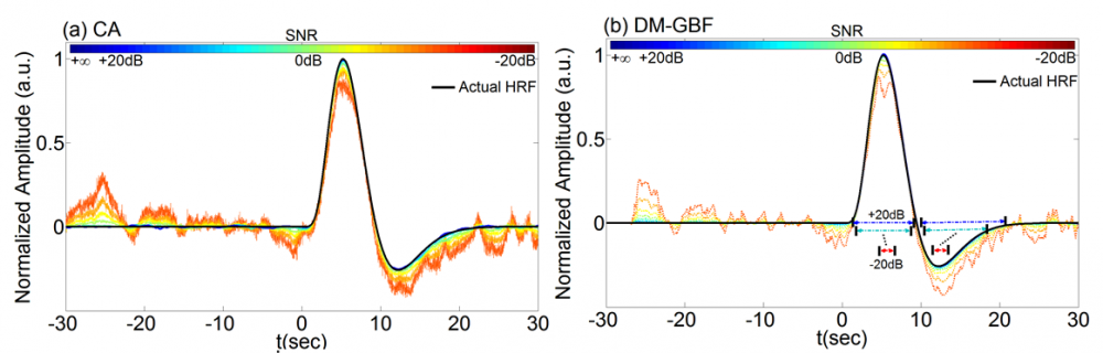
Figure 1. Average estimation results and root mean square error (RMSE) for Simulation 1 designed to investigate the effect of randomly spaced event sequences on the performance of CA and DM-GBF. In this simulation, NIRS signals were generated by using 2,000 uniformly distributed random events, synthesized random-phase physiological components and uncorrelated Gaussian random noise. Plots (a) and (b) illustrate the HRF profiles estimated by CA and DM-GBF, respectively, with SNRs ranging from -20 dB to +20 dB with 5 dB increments. In plot (b), the horizontal arrows indicate the time range over which gamma functions showed amplitudes (β coefficients) significantly (p<0.05) different from baseline. Simulation results were averaged over forty runs. CA: Conventional Averaging; DM-GBF: Deconvolution Model based on Gamma Basis Functions.
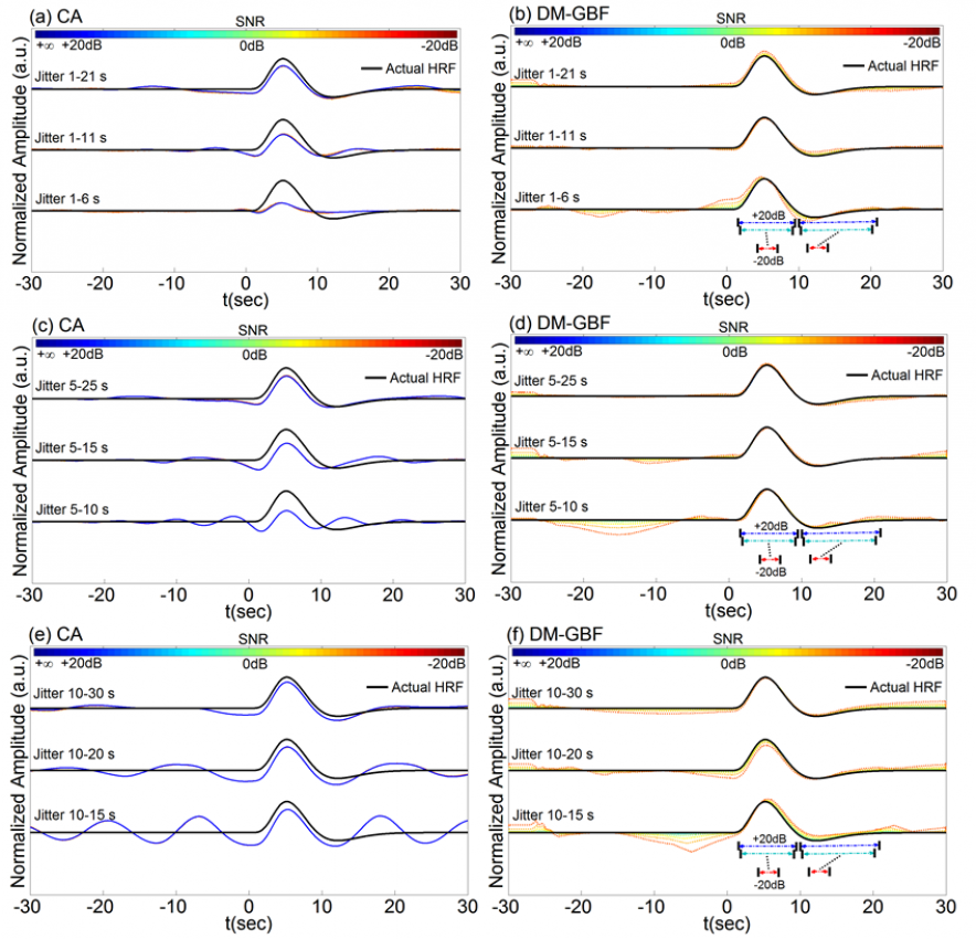
Figure 2. Average estimation results for Simulation 2 designed to investigate the effect of jittered event sequences on the performance of CA and DM-GBF. In this simulation, NIRS signals were generated by using 2,000 jittered events, synthesized random-phase physiological components and uncorrelated Gaussian random noise. Jittering was performed over 1-6 s, 1-11 s, 1-21 s, 5-10 s, 5-15 s, 5-25 s, 10-15 s, 10-20 s, or 10-30 s time intervals. Plots (a, c, e) illustrate the HRF profiles estimated by CA and DM-GBF, respectively, with SNRs ranging from -20 dB to +20 dB with 5 dB increments. In plot (b), the horizontal arrows indicate the time range over which gamma functions showed amplitudes (β coefficients) significantly (p<0.05) different from baseline. Simulation results were averaged over forty runs. CA: Conventional Averaging; DM-GBF: Deconvolution Model based on Gamma Basis Functions.
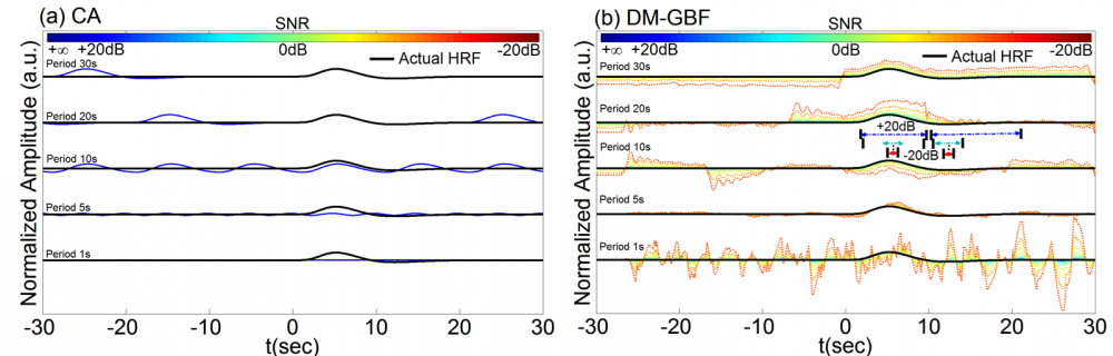
Figure 3. Average estimation results for Simulation 3 designed to investigate the effect of periodic event sequences on the performance of CA and DM-GBF. In this simulation, NIRS signals were generated by using five event sequences with 2,000 events regularly spaced over time with periods of 1s, 5s, 10s, 20s, and 30s, synthesized random-phase physiological components and uncorrelated Gaussian random noise. Plots (a and b) illustrate the HRF profiles estimated by CA and DM-GBF, respectively, with SNRs ranging from -20 dB to +20 dB with 5 dB increments. In plot (b), the horizontal arrows indicate the time range over which gamma functions showed amplitudes (β coefficients) significantly (p<0.05) different from baseline. Simulation results were averaged over forty runs. CA: Conventional Averaging; DM-GBF: Deconvolution Model based on Gamma Basis Functions.
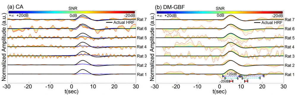
Figure 4. Average estimation results for Simulation 4 designed to investigate the effect of experimental event sequences on the performance of CA and DM-GBF. In this simulation, NIRS signals were generated by using experimental spike sequences (Rats 1-7) generated from the rat model of epilepsy, synthesized random-phase physiological components and uncorrelated Gaussian random noise. Plots (a) and (b) illustrate the HRF profiles estimated by CA and DM-GBF, respectively, with SNRs ranging from -20 dB to +20 dB with 5 dB increments. In plot (b), the horizontal arrows indicate the time range over which gamma functions showed amplitudes (β coefficients) significantly (p<0.05) different from baseline. Simulation results were averaged over forty runs. CA: Conventional Averaging; DM-GBF: Deconvolution Model based on Gamma Basis Functions.
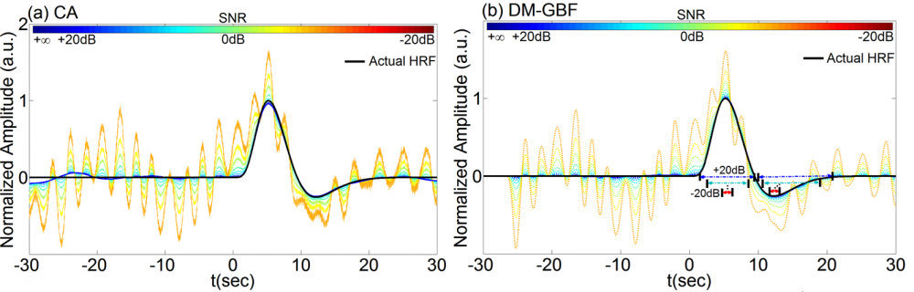
Figure 5. Average estimation results for Simulation 5 designed to investigate the effect of periodic physiological noise on the performance of CA and DM-GBF. In this simulation, NIRS signals were generated by using 2,000 uniformly distributed random events, synthesized periodic physiological components and uncorrelated Gaussian random noise. Plots (a) and (b) illustrate the HRF profiles estimated by CA and DM-GBF, respectively, with SNRs ranging from -20 dB to +20 dB with 5 dB increments. In plot (b), the horizontal arrows indicate the time range over which gamma functions showed amplitudes (β coefficients) significantly (p<0.05) different from baseline. Simulation results were averaged over forty runs. CA: Conventional Averaging; DM-GBF: Deconvolution Model based on Gamma Basis Functions.
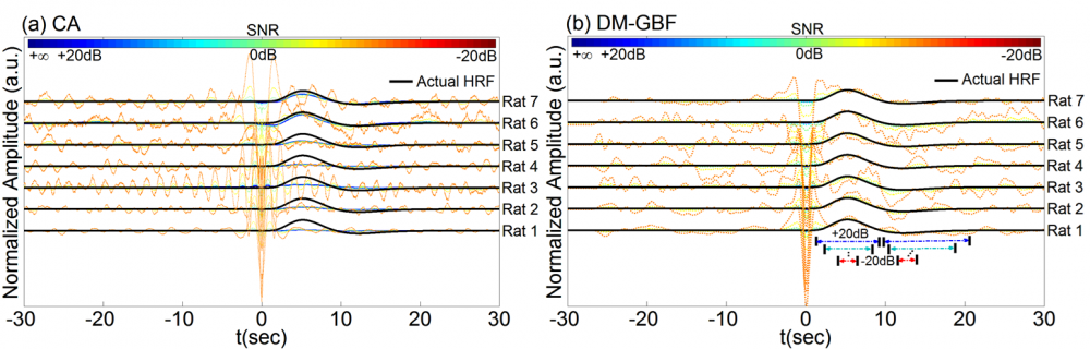
Figure 6. Estimation results for Simulation 6 designed to investigate the effect of phase-locked physiological noise on the performance of CA and DM-GBF. In this simulation, NIRS signals were generated by using experimental spike sequences (Rats 1-7) generated from the rat model of epilepsy, synthesized physiological components phase-locked to events and uncorrelated Gaussian random noise. Plots (a and b) illustrate the HRF profiles estimated by CA and DM-GBF, respectively, with SNRs ranging from -20 dB to +20 dB with 10 dB increments. In plot (b), the horizontal arrows indicate the time range over which gamma functions showed amplitudes (β coefficients) significantly (p<0.05) different from baseline. CA: Conventional Averaging; DM-GBF: Deconvolution Model based on Gamma Basis Functions.
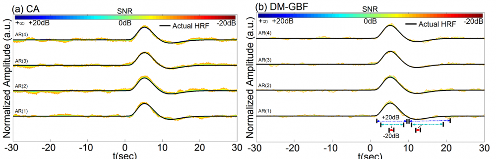
Figure 7. Average estimation results for Simulation 7 designed to investigate the effect of temporally correlated noise on the performance of CA and DM-GBF. In this simulation, NIRS signals were generated by using 2,000 uniformly distributed random events, synthesized random-phase physiological components and correlated Gaussian random noise with temporal correlations modeled with autoregressive (AR) models of orders 1-4. Plots (a) and (b) illustrate the HRF profiles estimated using CA and DM-GBF, respectively, with SNRs ranging from -20 dB to +20 dB with 5 dB increments. In plot (b), the horizontal arrows indicate the time range over which gamma functions showed amplitudes (β coefficients) significantly (p<0.05) different from baseline. Simulation results were averaged over forty runs. CA: Conventional Averaging; DM-GBF: Deconvolution Model based on Gamma Basis Functions.
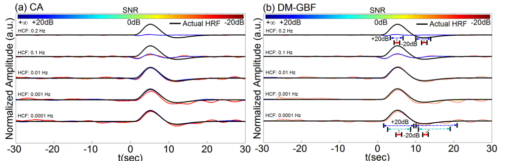
Figure 8. Average estimation results for Simulation 8-1 designed to investigate the effect of high-pass filtering on the performance of CA and DM-GBF. In this simulation, NIRS signals were generated by using 2,000 uniformly distributed random events, synthesized random-phase physiological components and uncorrelated Gaussian random noise. The resulting NIRS signals were then high-pass filtered with a high cut-off frequency (HCF) of 0.0001, 0.001, 0.01, 0.1 or 0.2 Hz. Plots (a and b) illustrate the HRF profiles estimated by CA and DM-GBF, respectively, with SNRs ranging from -20 dB to +20 dB with 10 dB increments. In plot (b), the horizontal arrows indicate the time range over which gamma functions showed amplitudes (β coefficients) significantly (p<0.05) different from baseline. Simulation results were averaged over forty runs. CA: Conventional Averaging; DM-GBF: Deconvolution Model based on Gamma Basis Functions.
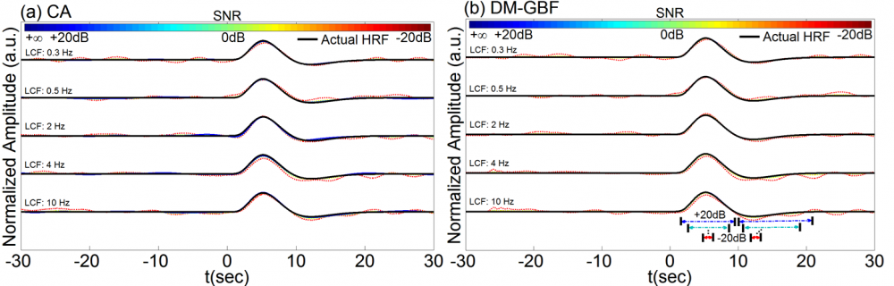
Figure 9. Average estimation results for Simulation 8-2 designed to investigate the effect of low-pass filtering on the performance of CA and DM-GBF. In this simulation, NIRS signals were generated by using 2,000 uniformly distributed random events, synthesized random-phase physiological components and uncorrelated Gaussian random noise. The resulting NIRS signals were then low-pass filtered with a low cut-off frequency (LCF) of 0.3, 0.5, 2, 4 or 10 Hz. Plots (a and b) illustrate the HRF profiles estimated using CA and DM-GBF, respectively, with SNRs ranging from -20 dB to +20 dB with 10 dB increments. In plot (b), the horizontal arrows indicate the time range over which gamma functions showed amplitudes (β coefficients) significantly (p<0.05) different from baseline. Simulation results were averaged over forty runs. CA: Conventional Averaging; DM-GBF: Deconvolution Model based on Gamma Basis Functions.
References
Aarabi, A., Osharina V., Wallois F., Effect of confounding variables on hemodynamic response function estimation using averaging and deconvolution analysis: An event-related NIRS study, Neuroimage, 2017.